General equilibrium

01/11/2024 - 01/30/24

Zihan

We have learned about the individual optimization and profit maximazition. In these problems, we typically take some elements as given. For example, in UMP, the prices are given. So, in these cases, we are actually looking for partial equilibrium.

Now, under a simple model, we work on a general equilibrium,

Pure exange economy

We have at least two goods.

For simplicity, we consider a static enviornment, in which transactions will not be repeated.

Agents: (individuals or households), indexed by $i=1,2,\dots ,I$$i = 1,2,\dots,I$

Goods: We have $L$$L$ goods, $l=1,2,\dots ,L$$l = 1,2,\dots, L$

Agents are characterized by

1. their consumption sets: $X_i\in {\mathbb{R}}_{+}^L$$X_i \in \R^L_+$, it has $L$$L$ dimensions and all elements are non-negative.

2. their preferences over consumption bundles in $X_i$$X_i$

   Preferences are represented by utility functions, namely $u:X_i\to \mathbb{R},\mathrm{\forall }i$$u:X_i \rightarrow \R, \forall i$.

   Utility functions need the utility function to be continuous, increasing, and semi quasi concave. (This one is Assumption 1)

3. Their endowments: $e_i\in {\mathbb{R}}_{++}^L$$e_i \in \R^L_{++}$, they are strictly positive for each element.

$x_i\in X_i$$x_i \in X_i$ represents each agent's consumption bundle, each $x_i=(x_{i1},x_{i2},\dots ,x_{iL}{)}^{\prime }$$x_i = (x_{i1},x_{i2},\dots,x_{iL})^\prime$.

We assume agents have competitive behavior, they take prices as given. (This means each one agent cannot change the price by himself, but this does not mean the price is exogeneously given).

We also assume agents are able to buy and sell any quantities of good they want, which means no friction

Definition 1. Allocation:

Allocation is a list $x=(x_1,x_2,\dots ,x_I)$$x = (x_1, x_2, \dots, x_I)$. Each element is the consumption bundle of agent $i$$i$,

We need the allocation to be feasible, which means it cannot exceed the aggregate number of endowments, i.e. $\sum _{i=1}^I{x}_i\le \sum _{i=1}^I{e}_i\in {\mathbb{R}}_{++}^L$$\sum_{i = 1}^I x_i \leq \sum_{i = 1}^I e_i \in \R^L_{++}$, where the LHS is the aggregate allocation, and the RHS is the aggregate endowments. NOTE that both $x_i$$x_i$ and $e_i$$e_i$ are vectors,

The leading example:

$I=2,L=2$$I = 2, L = 2$, we represent his economy with edgeworth box:

Definition 2. Pareto optimum.

A feasible allocation $x^{\ast }$$x^*$ is called Pareto Optimal if no another feasible allocation $x$$x$ such that :

Explanation to this defination:

For a feasible allocation $\mathbf{x}\in F(\mathbf{e})$$\mathbf{x} \in F(\mathbf{e})$

• It is Pareto efficient if there exists no other allocation $\mathbf{y}\in F(\mathbf{e})$$\mathbf{y} \in F(\mathbf{e})$ such that ${\mathbf{y}}^i\succsim {\mathbf{x}}^i$$\mathbf{y}^i \succsim \mathbf{x}^i$ for all consumers $i$$i$, with at least one preference relation strict ${\succ }_i$$\succ_i$.

• The process that an allocation $\mathbf{x}$$\mathbf{x}$ moves to $\mathbf{y}$$\mathbf{y}$ such that ${\mathbf{y}}^i\succsim {\mathbf{x}}^i$$\mathbf{y}^i \succsim \mathbf{x}^i$ for all consumers $i$$i$, with at least one preference relation strict ${\succ }_i$$\succ_i$ is called Pareto improvement.

• In other word, an allocation is Pareto efficient if there is no Pareto improvement.

Graphical presentation: Contract curve

• All Pareto efficient allocation in Edgeworth box.

• Special cases: prefect substitutes; perfect complements

  

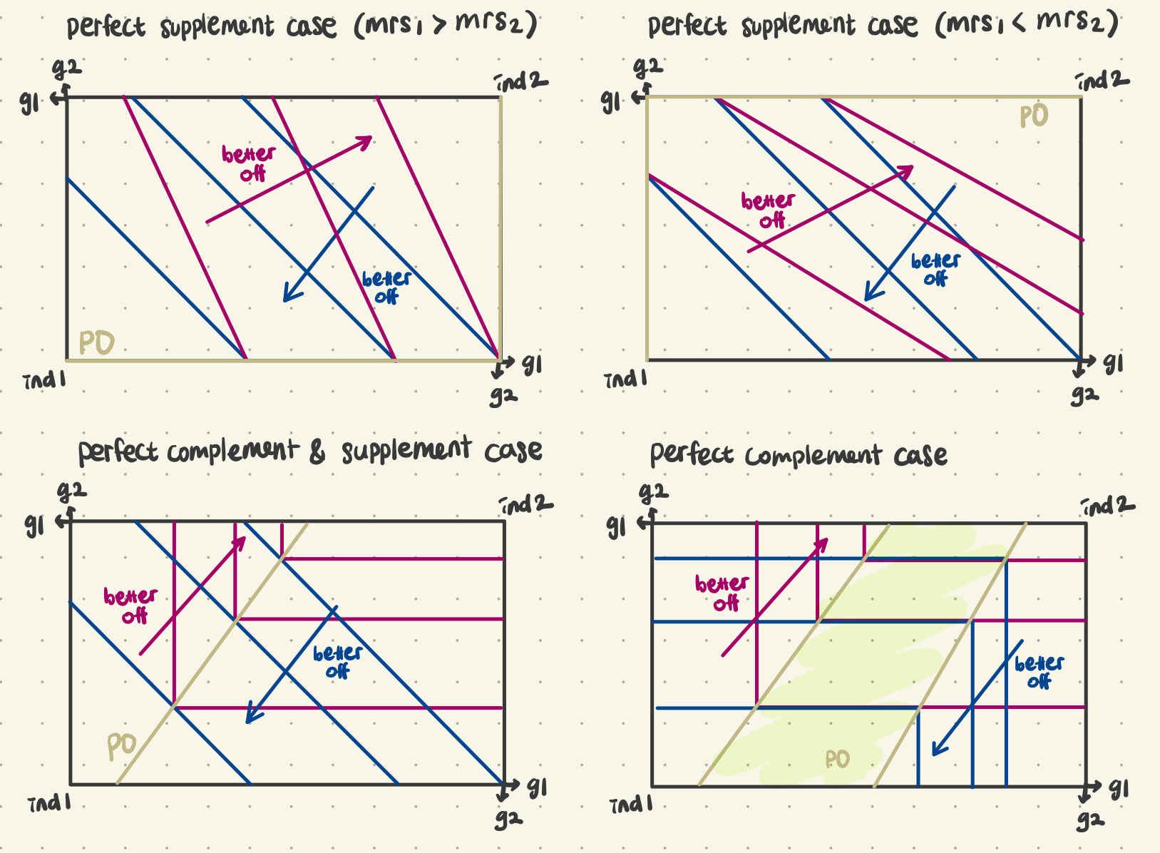
For smooth IC curves, PO allocation one points of tangetly btw IC curves

Problems with PO allocation,

1. we cannot rank them

2. we cannot always even rank PO allocation versus non PO allocations

3. An allocation where one agent gets all the resources is a PO.

Definition3. Competitive

An allocation $x$$x$ is called competitive if $\mathrm{\exists }p\in {\mathbb{R}}_{+}^L$$\exist p \in \R^L_+$ (without 0), such that,

1. Given $p$$p$ for every $i$$i$, $x_i$$x_i$ is a solution to

   $$\begin{array}{}\text{(2)}& max{u}_i(x_i)s.t.p(x_i-e_i)\le 0\end{array}$$

2. market clearing conditions

   $$\begin{array}{}\text{(3)}& \begin{array}{c}\sum _{i=1}^I{x}_i(p)=\sum _{i=1}^I{e}_i\text{w/o free disposal}\\ \sum _{i=1}^I{x}_i(p)\le \sum _{i=1}^I{e}_i\text{with free disposal}\end{array}\end{array}$$

An example

Definition: Compatitive equilibrium /Walrasian equilibrium

A competitive (Walrasian) equilibrium is a pair $(p,x)$$(p,x)$ where $x$$x$ is a competitive allocation for $p$$p$​

Then we have several famous theorems

• [First welfare theorem]: Every competitive allocation is a Pareto Optimum (PO)

• [Second welfare theorem]: Any PO allocation can be supported (reached) by with some dedistribution of resources.

Another example

Suppose the utilitty for two consumers are

$$\begin{array}{}\text{(4)}& u_i(x_{1i},x_{2i})=x_{1i}^{\alpha }{x}_{2i}^{1-\alpha }\end{array}$$

Endowments： $e_1=(1,2),e_2=(2,1)$$e_1 = (1,2), e_2 = (2,1)$,

How do we derive the competitive equilibrium?

Given $p=(p_1,p_2)$$p = (p_1, p_2)$, individual 1 solves

$$\begin{array}{}\text{(5)}& \begin{array}{c}max{x}_{1i}^{\alpha }{x}_{2i}^{1-\alpha }\\ s.t.p_1{x}_{11}+p_2{x}_{21}\le p_1+2p_2\end{array}\end{array}$$

By solving this UMP problem,

$$\begin{array}{}\text{(6)}& \begin{array}{rl}{x}_{11}^{\ast }& =\frac{\alpha (p_1+2p_2)}{p_1}\\ x_{21}^{\ast }& =\frac{(1-\alpha )(p_1+2p_2)}{p_2}\end{array}\end{array}$$

We can solve the same UMP problem for individual 2 as well,

$$\begin{array}{}\text{(7)}& \begin{array}{rl}{x}_{12}^{\ast }& =\frac{\alpha (2p_1+p_2)}{p_1}\\ x_{22}^{\ast }& =\frac{(1-\alpha )(2p_1+p_2)}{p_2}\end{array}\end{array}$$

Then, applying the market clearing condition, what we obtained is,

$$\begin{array}{}\text{(8)}& \frac{\alpha (p_1+2p_2)}{p_1}+\frac{\alpha (2p_1+p_2)}{p_1}=3\end{array}$$

and,

$$\begin{array}{}\text{(9)}& \frac{(1-\alpha )(p_1+2p_2)}{p_2}+\frac{(1-\alpha )(2p_1+p_2)}{p_2}=3\end{array}$$

Two equations above give the same result of price ratio.

$$\begin{array}{}\text{(10)}& \frac{p_2}{p_1}=\frac{1-\alpha }{\alpha }\end{array}$$

subsitute this result back to the demand function, we can get the number of demand for each individual under this endowment.

Here in this example, we did something redundant. Actually we just need one market to be clear, and the other one will be automatically clear as well.

Given endowment $e$$e$, let $F(e)$$F(e)$ be the set of feasible allocations

Definition. Feasible allocation and "block"

Let $\overline{I}\subseteq I$$\bar I \subseteq I$ and $x\in F(e)$$x \in F(e)$, $\overline{I}$$\bar I$ blocks $x$$x$ if there is another allocation $y$$y$ such that, (Here set $\overline{I}$$\bar I$ is individuals).

• $\sum _{i\in \overline{I}}{y}_i=\sum _{i\in \overline{I}}{e}_i$$\sum_{i \in \bar I} y_i = \sum_{i \in \bar I}e_i$, this means that this allocation $y$$y$ is feasible

• Under an another allocation, it could be slightly better, i.e. $y_i{\succsim }_i{x}_i,\mathrm{\forall }i\in \overline{I}$$y_i \succsim_i x_i, \forall i \in \bar I$, and $y_j{\succ }_j{x}_j$$y_j \succ_j x_j$ for at least one $j\in \overline{I}$$j \in \bar I$.

  如果一个allocation $x$$x$ 存在帕累托改进 ，say new allocation $y$$y$，那么这个 $x$$x$ will be blocked by these two individuals.

  但是即使是Pareto optimum，它这个allocation 仍然可以被其中一个人block。(block by one individual)

Definition. Core

The core of an exchange economy with endowment $e$$e$ , denoted by $C(e)$$C(e)$, is the set of all unblocked feasible allocations. In other words, an allocation $x\in F(e)$$x \in F(e)$ is in core if no subset of individuals can block it.

推论：Show that $C(e)\subseteq PO(e)$$C(e) \subseteq PO(e)$ , explain it in own words. Everyone in the "core" is a pareto optimum

Suppose there exists a feasible allocation $x\in F(e)$$x \in F(e)$ such that $x\in C(e)$$x \in C(e)$ but $x\notin PO(e)$$x \not \in PO(e)$.

Therefore, by definition of Pareto Optimum, there exists a feasible allocation $x^{\ast }$$x^*$ such that $\mathrm{\forall }i{u}_i(x_i)\ge u_i(x_i^{\ast })$$\forall i \quad u_i(x_i) \geq u_i(x_i^*)$, but some $u_i(x_i)>u_i(x_i^{\ast })$$u_i(x_i) > u_i(x_i^*)$, which has the same meaning of $\mathrm{\forall }i,x_i^{\ast }\succsim x_i^{\ast }$$\forall i, x^*_i \succsim x^*_i$, and for some $i$$i$, $y_i\succ x_i$$y_i \succ x_i$. Hence, we know that $x^{\ast }\notin C(e)$$x^* \not \in C(e)$, which is contradictory to $x\in C(e)$$x \in C(e)$.

Hence, whenever $x\in C(e)$$x \in C(e)$, $x\in PO(e)$$x \in PO(e)$, which implies $C(e)\subseteq PO(e)$$C(e) \subseteq PO(e)$.

Recall that we assume agent's utility function satisfies continuity, semi quasi concavity and increasing (strictly increasing), (This is assumption 1).

Each individual is price taker. Given $p>>0$$p >> 0$, each individual problem is

when $u_i$$u_i$ satisfies assumption 1, there is a unique solution to individual's utility maximization. i.e. $x_i(p)$$x_i(p)$ is unique and continuous when $p>>0$$p >> 0$.

Existance of $x_i(p)$$x_i(p)$ follows from boundedness of budget set and uniqueness follows from s.q. concavity.

Individual $i$$i$'s excess demand for good $l$$l$ is $z_i^l(p)=x_i^l(p)-e_i^l$$z_i^l(p) = x_i^l(p) - e_i^l$.

Aggregate excess demand for good $l$$l$ is

Theorem - Walras law

Let $z(p)\in {\mathbb{R}}^L$$z(p) \in \R^L$ If $u_i$$u_i$ satisfies Assumption 1, then $pz(p)=0$$p z(p) = 0$

This actually means that the value of aggregate excess demand will always be zero at any set of positive prices.

Proof

By Assumption 1, It implies budget constraint holds with equality for all $i\in \overline{I}$$i \in \bar I$​,

$$\begin{array}{}\text{(13)}& \sum _{l=1}^L{p}_l{x}_i^l(p)=\sum _{l=1}^L{p}_l{e}_i^l\end{array}$$

Then,

$$\begin{array}{}\text{(14)}& \sum _l^L{p}_l(x_i^l(p)-e_i^l)=0\end{array}$$

Thus, if we aggregate over all the individuals it becomes, (note that the order of summation is not important)

$$\begin{array}{}\text{(15)}& \begin{array}{c}\sum _{i\in \overline{I}}\sum _l^L{p}_l(x_i^l(p)-e_i^l)=0\\ \sum _l^L\sum _{i\in \overline{I}}{p}_l(x_i^l(p)-e_i^l)=0\\ \sum _l^L{p}_l\sum _{i\in \overline{I}}\underset{\text{Excess demand for good }l:z_i^l(p)}{\underbrace{(x_i^l(p)-e_i^l)}}=0\end{array}\end{array}$$

Then we obtained what we wanna prove:

$$\begin{array}{}\text{(16)}& \sum _l{p}_l{z}_l(p)=pz(p)=0\end{array}$$

An immediate implication of the walres law is that the following:

If given some set of prices that are strictly positive, if $L-1$$L - 1$ martets are in equilibrium (clear), then the $L$$L$ market will also be clear (in equilibrium).

Definition - Walrasian equilibrium

A vector of prices $p^{\ast }\in {\mathbb{R}}_{++}^L$$p^*\in \R^L_{++}$ is called Walrasian equilibrium if $z(p^{\ast })=0$$z(p^*) = 0$

Walrasian equilibrium 定义的是价格。它使所有商品都不存在超额需求/供给

In this definition, we define equilibrium as price vector. However, the allocation $x(p^{\ast })$$x(p^*)$ implicitly consistent with the equilibrium itself, as a result, we represent walrasian equilivbrium as $(x(p^{\ast }),p^{\ast })$$(x(p^*), p^*)$

Theorem - Existance of Walrasian equilibrium,

If each individual's utility function satisfies Assumption 1, and $\sum _{i=1}^I{e}_i>>0$$\sum_{i = 1}^I e_i >>0$, then there exists at least one price vector $p^{\ast }>>0$$p^*>>0$, such that , $z(p^{\ast })=0$$z(p^*) = 0$ , which implies that the Walresian equilibrium exists.

Definition. [Walrasian allocation] - Given Walrasian equilibrium price $p^{\ast }$$p^*$, let $x_k(p^{\ast })$$x_k(p^*)$ be the goods received by $k$$k$th individual under this economy, then

is the Walrasian equilibrium allocation.

From this, we have two observations.

• Observation 1let $e$$e$ be endowment and $p^{\ast }$$p^*$ be Walrasian equilibrium and $x(p^{\ast })$$x(p^*)$ be WE allocation, then $x(p^{\ast })\in F(e)$$x(p^*) \in F(e)$.

  Proof

  For homework!

  Suppose $p^{\ast }$$p^*$ is a Walrasian equilibrium, and $x^{\ast }=x(p^{\ast })$$x^* = x(p^*)$ is the corresponding Walrasian allocation. and $x(p^{\ast })$$x(p^*)$ is not feasible. So we have $\sum _{i=1}^I{x}_i^{\ast }>\sum _{i=1}^I{e}_i\in {\mathbb{R}}_{++}^L$$\sum_{i = 1}^I x_i^* > \sum_{i = 1}^I e_i \in \R^L_{++}$, which means that $z(p^{\ast })=\sum _{i=1}^I{x}_i^{\ast }-e_i>{\mathbf{0}}^L$$z(p^*) = \sum_{i = 1}^I x_i^* - e_i > \bold 0^L$, which violates the definition of Walrasian allocation that $z(p^{\ast })=0$$z(p^* ) = 0$. Contradiction! So any Walrasian equilibrium must be an feasible allocation.

   

• Observation 2 $u_i$$u_i$ is strictly increasing, and $p>>0$$p>>0$​,

  • if $u_i(x_i^{\prime })>u_i(x_i(p))$$u_i(x_i^\prime) > u_i(x_i(p))$, then $p{x}_i^{\prime }>p{x}_i(p)=p{e}_i$$p x_i^\prime > p x_i(p) = pe_i$

    This looks quite similar to WARA, if there is some better off utility allocation, it cannot be affordable.

  • if $u_i(x_i^{\prime })\ge u_i(x_i(p))$$u_i(x_i^\prime ) \geq u_i(x_i(p))$, then $p{x}_i^{\prime }\ge p{x}_i(p)$$p x_i^\prime \geq px_i(p)$

    Proof

    For homework.

    We wanna show hat if $p{x}_i^{\prime }<p{x}_i(p)$$p x_i^\prime < px_i(p)$, then $u_i(x_i^{\prime })<u_i(x_i(p))$$u_i(x_i^\prime ) < u_i(x_i(p))$,

    Suppose there exists some new allocation such that $p{x}_i^{\prime }<p{x}_i(p)$$p x_i^\prime < px_i(p)$, but $u_i(x_i^{\prime })\ge u_i(x_i(p))$$u_i(x_i^\prime ) \geq u_i( x_i(p))$, therefore, let $x_i^{\prime \prime }=({x_i^1}^{\prime }+{ϵ}^1,\dots ,{x_i^L}^{\prime }+{ϵ}^L)$$x_i^{\prime \prime } = ({x_i^1} ^\prime + \epsilon^1, \dots, {x_i^L} ^\prime + \epsilon^L)$, where ${ϵ}^l$$\epsilon^l$ are some small numbers, then there could be some $x_i^{\prime \prime }$$x_i^{\prime \prime }$ such that $p{x}_i^{\prime }<p{x}_i^{\prime \prime }<p{x}_i(p)$$p x_i^\prime < px_i^{\prime \prime} < px_i(p)$ and $u_i(x_i^{\prime \prime })>u_i(x_i^{\prime })\ge u_i(x_i(p))$$u_i (x_i^{\prime \prime })> u_i(x_i^\prime ) \geq u_i( x_i(p))$ because $u_i$$u_i$ is assumed to be strictly increasing. Therefore, it contradicts with the statement of if $u_i(x_i^{\prime \prime })>u_i(x_i(p))$$u_i(x_i^{\prime \prime}) > u_i(x_i(p))$, then $p{x}_i^{\prime \prime }>p{x}_i(p)=p{e}_i$$p x_i^{\prime \prime}> p x_i(p) = pe_i$. $◻$$\square$

Let $W(e)$$W(e)$ be the set of Walrasian equilibrium allocations given $e$$e$​.

Theorem

Let $u_i$$u_i$ be strictly increasing on ${\mathbb{R}}_{+}^L$$\R_+^L$ and $e$$e$ be endowment vector,

This implies that every WE alllcation is in the core.

Proof

Proof by contradiction,

On the contrary, there exist $p^{\ast }$$p^*$ such that $x(p^{\ast })\in W(e)$$x(p^*) \in W(e)$ and $x(p^{\ast })\notin C(e)$$x(p^*) \not \in C(e)$,

Since $x(p^{\ast })$$x(p^*)$ is Waralsian equailibrium allocation, then from the oberservation 1, $x(p^{\ast })\in F(e)$$x(p^*) \in F(e)$, it is a feasible allocation.

Then there exists an alternative allocation $y$$y$ and a subset of individuals $\overline{I}$$\bar I$, such that $\overline{I}$$\bar I$ blocks $x(p^{\ast })$$x(p^*)$ with $y$$y$.

That is $\sum _{i\in \overline{I}}{y}_i=\sum _{i\in \overline{I}}{e}_i$$\sum_{i \in \bar I} y_i = \sum_{i \in \bar I} e_i$, $u_i(y_i)\ge u_i(x_i(p^{\ast }))$$u_i(y_i)\geq u_i(x_i(p^*))$ for all $i\in \overline{I}$$i\in \bar I$, and $u_j(y_j)>u_j(x_j(p^{\ast }))$$u_j(y_j) > u_j(x_j(p^*))$ for some $i$$i$.

We can multiply both sides of $\sum _{i\in \overline{I}}{y}_i=\sum _{i\in \overline{I}}{e}_i$$\sum_{i \in \bar I} y_i = \sum_{i \in \bar I} e_i$ with $p^{\ast }$$p^*$, then it becomes $p^{\ast }\sum _{i\in \overline{I}}{y}_i=p^{\ast }\sum _{i\in \overline{I}}{e}_i$$p^* \sum_{i \in \bar I} y_i = p^* \sum_{i \in \bar I} e_i$.

And from Observation 2, $p{y}_i>p{x}_i(p)=p{e}_i$$p y_i > p x_i(p) = pe_i$ for all $i\in \overline{I}$$i \in \bar I$, and $p^{\ast }{y}_j>p^{\ast }{x}_j(p^{\ast })=p^{\ast }{e}_j$$p^* y_j > p^*x_j(p^*) = p^* e_j$ for some $j\in \overline{I}$$j \in \bar I$, we sum up all individuals in $\overline{i}$$\bar i$,

$p^{\ast }\sum _{i\in \overline{I}}{y}_i>p^{\ast }\sum _{i\in \overline{I}}{e}_i$$p^*\sum_{i\in \bar I} y_i > p^* \sum_{i\in \bar I} e_i$, there is a contradiction.

$◻$$\square$

Definition

Let $e$$e$ be endowment vector, a feasible allocation $x^{\ast }\in F(e)$$x^* \in F(e)$ is Pareto Optimal if there does not exist another feasible allocation $y\in F(e)$$y \in F(e)$, such that,

Suppose $L=2$$L=2$, we can define the set of PEAs as the vector $(x_1,\dots ,x_I)$$(x_1, \dots, x_I)$, that solves

Note that here each $x_i$$x_i$ is a vector has $L$$L$ dimensions (goods).

This allocation $(x_1,\dots ,x_I)$$(x_1, \dots, x_I)$​ is PE if it maximizes individual 1's utility without reducing the utility of all other individuals below a given utility level, and satisfying the feasiblity condition.

The lagrange function should be like,

FOCs for interior solution give (Here $x_j^1$$x_j^1$ represents the first good of individual $j$$j$ has )

Example

Two individuals $A$$A$ and $B$$B$, there are two goods 1 and goods 2.

Say the endowment: $e_A=(100,350)$$e_A = (100, 350)$ and $e_B=(100,50)$$e_B = (100, 50)$.

And the utility function $U_A=x_A^1{x}_A^2$$U_A = x_A^1 x_A^2$ and $U_B=x_B^1{x}_B^2$$U_B = x_B^1 x_B^2$. Find the PEA.

For Agent $A$$A$,

$$\begin{array}{}\text{(23)}& \begin{array}{rl}\underset{x_A^1,x_A^2,x_B^1,x_B^2}{max}& x_A^1{x}_A^{2}s.t.\\ & x_B^1{x}_B^2\ge {\overline{u}}_B\\ & x_A^1+x_B^1=200\\ & x_A^2+x_B^2=400\end{array}\end{array}$$

Then,

$$\begin{array}{}\text{(24)}& \mathcal{L}=x_A^1{x}_A^2-\lambda (x_B^1{x}_B^2-{\overline{u}}_B)-{\mu }_1(200-x_A^1-x_B^1)-{\mu }_2(400-x_A^2-x_B^2)\end{array}$$

FOCs:

$x_A^1:x_A^2-{\mu }_1=0$$x_A^1: x_A^2 - \mu_1 = 0$,

$x_A^2:x_A^1-{\mu }_2=0$$x_A^2: x_A^1 - \mu_2 = 0$,

$x_B^1:\lambda x_B^2-{\mu }_1=0$$x_B^1: \lambda x_B^2 - \mu_1 =0$

$x_B^2:\lambda x_B^1-{\mu }_2=0$$x_B^2: \lambda x_B^1 - \mu_2 = 0$

This implies,

$$\begin{array}{}\text{(25)}& \frac{x_A^2}{x_A^1}=\frac{{\mu }_1}{{\mu }_2}=\frac{x_B^2}{x_B^1}\end{array}$$

Substitute with some budget constraints,

$$\begin{array}{}\text{(26)}& \frac{x_A^2}{x_A^1}=\frac{400-x_A^2}{200-x_A^1}\end{array}$$

, which gives us $x_A^2=2x_A^1$$x_A^2 = 2x_A^1$​ describing the PEA.

In Walrasian equilibrium, each individual wants to choose a bundle that maximizes their own utility, She knows nothing about other individuals. By showing WEA is in the core, we have shown that it is possible to believe outcomes in the core without a central planner, which means the market works. that is because

Theorem - First Welfare theorem

If each individual's utility is strictly increasing that every WEA is pareto equilibrium.

Question: Can we consider a WEA as equitable or socially optimal?

• It is clear that if an allocation is not pareto efficient, than not socially optimal.

  

Theorem - Second Welfare theorem

Let $e$$e$ be the initial endowment with $\sum _{i=1}^I{e}_i>>0$$\sum_{i =1}^I e_i >>0$, let $u_i$$u_i$ satisfy assumption 1 for all individuals, let $\overline{x}$$\bar x$ be a PEA for $(u_i{)}_{i\in I}$$(u_i)_{i\in I }$ and $e$$e$, then $\overline{x}$$\bar x$ is the unique WEA for economy $(u_i{)}_{i\in I}$$(u_i)_{i\in I}$, $e=\overline{x}$$e = \bar x$

Proof

Since $\overline{x}$$\bar x$ is PE, $\overline{x}\in F(e)\Rightarrow \sum _i^I{\overline{x}}_i=\sum _i^I{e}_i>>0$$\bar x \in F(e) \Rightarrow \sum_i^I \bar x_i = \sum_i^I e_i >>0$,

Since $u_i$$u_i$ satisfies Assumption 1, then for all $i\in I$$i \in I$, and $\sum _{i\in I}{\overline{x}}_i>>0$$\sum_{i \in I} \bar x_i>>0$, the existence of WEA for $e^{\prime }=\overline{x}$$e^\prime = \bar x$ and $(u_i{)}_{i\in I}$$(u_i)_{i\in I }$ is guaranteed. Let $\hat{x}$$\hat x$ ($\hat{x}\in F(e^{\prime })$$\hat x \in F(e^\prime )$)be WEA for economy $(u_i{)}_{i\in I}$$(u_i)_{i\in I}$ and $e^{\prime }=\overline{x}$$e^\prime = \bar x$,

Since under WEA each individual maximizes utilitty given initial endowment, we have,

$$\begin{array}{}\text{(28)}& u_i({\hat{x}}_i)\ge u_i(e_i^{\prime })=u_i({\overline{x}}_i),\mathrm{\forall }i\in I\end{array}$$

Since $\hat{x}\in F(e^{\prime })=F(\overline{x})=F(e)$$\hat x \in F(e^\prime ) = F(\bar x) = F(e)$, we have

$$\begin{array}{}\text{(29)}& \sum _{i\in I}{\hat{x}}_i=\sum _{i\in I}{\overline{x}}_i=\sum _{i\in I}{e}_i\end{array}$$

Since $\overline{x}$$\bar x$ is PEA, $\hat{x}$$\hat x$ cannot Pareto dominate $\overline{x}$$\bar x$ (That means no $j\in I$$j\in I$ such that $u_j({\hat{x}}_j)>u_j({\overline{x}}_j)$$u_j(\hat x_j )> u_j(\bar x_j)$),

Then $u_i({\hat{x}}_i)=u_i({\overline{x}}_i)\mathrm{\forall }i\in I$$u_i(\hat x_i ) = u_i(\bar x_i) \quad \forall i \in I$,

Suppose ${\hat{x}}_i\ne {\overline{x}}_i$$\hat x_i \neq \bar x_i$ for some $i$$i$,

if ${\hat{x}}_i>>{\overline{x}}_i$$\hat x_i >> \bar x_i$ then some $u_i$$u_i$ is strictly increasing, then $u_i({\hat{x}}_i)>u_i({\overline{x}}_i)$$u_i(\hat x_i ) > u_i(\bar x_i)$, contradict!

Then ${\hat{x}}_i^k>{\overline{x}}_i^k$$\hat x_i^k > \bar x_i^k$ and ${\hat{x}}_i^{k^{\prime }}<{\overline{x}}_i^{k^{\prime }}$$\hat x_i^{k^\prime } < \bar x_i^{k^\prime }$,

Then for ${\hat{x}}_i^k>{\overline{x}}_i^k$$\hat x_i^k > \bar x_i^k$ and ${\overline{x}}_i^{k^{\prime }}>{\hat{x}}_i^{k^{\prime }}$$\bar x_i^{k^\prime} > \hat x_i^{k^\prime}$, for some $k,k^{\prime }\in L$$k , k^\prime \in L$, (For simplicity let $i,j$$i,j$ be the only individuals ${\hat{x}}_j^k<{\overline{x}}_j^k$$\hat x_j ^k < \bar x_j^{k }$ and ${\hat{x}}_j^{k^{\prime }}>{\overline{x}}_j^{k^{\prime }}$$\hat x_j ^{k^\prime} > \bar x_j^{k^\prime }$),

Then by strict quasi concavity, by averaging bundles ${\overline{x}}_i$$\bar x_i$ and ${\hat{x}}_i$$\hat x_i$, i can have a new bundle ${\tilde{x}}_i$$\tilde x_i$, which gives a higher utility which is a contradiction.

$◻$$\square$

A short summary for welfare theorems

Walrasian equilibrium allocation (WEA)

$$\begin{array}{}\text{(30)}& \mathbf{x}\left({\mathbf{p}}^{\ast }\right)=({\mathbf{x}}^1({\mathbf{p}}^{\ast },{\mathbf{p}}^{\ast }\cdot {\mathbf{e}}^1),\dots ,{\mathbf{x}}^I({\mathbf{p}}^{\ast },{\mathbf{p}}^{\ast }\cdot {\mathbf{e}}^1))\in F(\mathbf{e})\end{array}$$

First welfare theorem: Walrasian Equilibrium $\to$$\rightarrow$ Pareto efficiency

• No distortion of price

• No externalities

• No asymmetric information

• No market power

Second welfare theorem:

Any Pareto efficient allocation can result from a Walrasian equilibrium (given that endowments can be redistributed in a lump sum way)

Example

let $u_A=x_A^1{x}_A^2$$u_A = x_A^1 x_A^2$ and $u_B=min\{x_B^1,x_B^2\}$$u_B = \min \left\{ x_B^1, x_B^2\right\}$. $e_A=(1,3)$$e_A=(1,3)$, $e_B=(3,1)$$e_B = (3,1)$​

Show Edgeworth box, find out PEA, find out WEA, and the prices

This economy in edgeworth box is

For the WEAs, we have to solve the UMP given endowments.

Homework

1. change the $e_A=(4,1)$$e_A = (4,1)$ and $e_B=(2,3)$$e_B = (2,3)$​​, show PEA in this economy

   

2. $$\begin{array}{}\text{(31)}& \begin{array}{c}{U}^A(x_A,y_A)=x_A+(y_A+0.5{)}^{0.5}\\ U^B(x_B,y_B)=x_B+y_B+1/4\\ e_A=e_B=(1,1)\end{array}\end{array}$$

3.  

First derive the WEA,

For agent $A$$A$

$$\begin{array}{}\text{(32)}& \begin{array}{rl}max{U}^A(x^A,y^A)& =x_A+{(y_A+0.5)}^{0.5}\\ \text{ s.t. }P{x}_A+y_A& =p+1\end{array}\end{array}$$

Then,

$$\begin{array}{}\text{(33)}& \mathcal{L}=x_A+{(y_A+0.5)}^{0.5}-\lambda (p{x}_A+y_A-p-1)\end{array}$$

The first order conditions are:

• $1-\lambda p=0$$1-\lambda p = 0$

• $0.5{(y_A+0.5)}^{-0.5}-\lambda =0$$0.5\left(y_A+0.5\right)^{-0.5}-\lambda=0$​

Then $0.5(y_A+0.5{)}^{-0.5}=\frac{1}{p}$$0.5(y_A+0.5)^{-0.5}=\frac{1}{p}$, which implies,

$$\begin{array}{}\text{(34)}& \begin{array}{rl}& y_A=\frac{p^2}{4}-\frac{1}{2}\\ & x_A=-\frac{p}{4}+\frac{3}{2p}+1\end{array}\end{array}$$

For agent B, he maximizes

$$\begin{array}{}\text{(35)}& \begin{array}{rl}max{U}^B(x^B,y^B)& =x_B+y_B\\ \text{ s.t. }p{x}_B+y_B& =p+1\end{array}\end{array}$$

Since the utility function is linear, we have to discuss by case.

• If $p<1$$p<1$, then $x_B=\frac{p+1}{p}$$x_B = \frac{p+1}{p}$, and $y_B=0$$y_B = 0$

  In this case, by the market clearing condition, $x_A+x_B=2$$x_A + x_B = 2$, we derive $p=\sqrt{10}$$p = \sqrt{10}$, which does not make sense.

• If $p>1$$p > 1$, then $x_B=0$$x_B = 0$, and $y_B=p+1$$y_B = p+1$,

  In this case, by the market clearing condition, $x_A+x_B=2$$x_A + x_B = 2$, $p=\sqrt{10}-2>1$$p = \sqrt{10} - 2 >1$. So it could be the WEA.

• If $p=1$$p = 1$, then $x_B+y_B=1+p$$x_B + y_B = 1+p$, but we have $y_A<0$$y_A<0$ under this price, so it could not be a feasible allocation under this price $p=1.$$p = 1.$

In summary, the WEA is $p=\sqrt{10}-2$$p = \sqrt{10}-2$.

Then, the PEA

The Green curve represents the PEA in the edgeworth box. All these POs lie on the edge of the box.

Incorporating Production

We have production in the economy, but let's first consider the most simpliest Rubison economy

There is a firm producing coconut, selling it to Rubison and make profits. Rubison sells labor to the firm.

Say the production function is,

Say Rubinson's utility is,

, where $h$$h$ is the leisure, and $c$$c$ is consumption of coconuts.

Rubinson has $T$$T$ hours to allocate, and let's say the initial endowment $e_c=0$$e_c = 0$, (No coconut at the beginning) and $e_h=T$$e_h = T$.

Then the budget constraints for Robinson are,

Then, we can set the largrange by,

Here we know that actuall $\mu =0$$\mu = 0$ has to be satisfied because whenever it does not, $T=h$$T = h$, and there is no production, no profit and then no consumption. Then utilitty will be zero, this is inferior.

So $\mu =0$$\mu=0$, and our largrange function becomes,

The first-order conditions are,

• ${\mathcal{L}}_h=(1-\beta )h^{-\beta }{c}^{\beta }-\lambda P_h=0$$\mathcal L_h = (1-\beta ) h^{-\beta} c^\beta - \lambda P_h = 0$

• ${\mathcal{L}}_c=\beta h^{1-\beta }{c}^{\beta -1}-\lambda P_c=0$$\mathcal L_c = \beta h^{1-\beta }c ^{\beta-1} - \lambda P_c = 0$

• $\lambda (P_{h}T+{\pi }^{\ast }-P_{c}c-P_{h}h)=0$$\lambda(P_h T + \pi^* -P_c c- P_hh) = 0$

Then we know the last constraint must be binding, and the solve for the first order conditions, l

Then combine with the budget constraint, we can derive the Rubinson's marshalian demand for coconut and labor,

(Here $h$$h$ denotes leisure demand, but in the producer problem $h$$h$ denotes labor )

Next lets consider the producer's problem. (profit max problem)

Then solve this problem, it gives us firm's demand on labor

And we can derive the profit as well

For completely solving the market equilibrium (general equilibrium), we need to consider the market clearing condition after deriving the partial equilibrium of these two markets.

Labor market clearing: labor demand = labor supply (leisure + labor. = T)

, which gives us $P_h=1,P_c=\sqrt{\frac{4\beta T}{2-\beta }}$$P_h = 1, P_c = \sqrt{\frac{4\beta T}{2-\beta }}$.

Exams on Feb. 8, TA sessions on Friday.